A step-by-step account of tuning cpu and memory use for a Spark job on Kubernetes

In our experience, software developers rarely plan the future memory needs of their apps while they’re building them. What usually happens is that once apps go live, data begins to grow and the system is tweaked and tuned to the limit until an entire new memory model is eventually needed. In the interim, quite a bit of memory, compute power, and money are wasted.

Because predicting future memory requirements is so complex, most efforts to optimize usually assume only the most common use cases. We can all do better. 

Here we demonstrate a methodology for troubleshooting and optimizing memory and other resource efficiency during the testing phases of Apache Spark jobs. 

First things first – plan for growth.

How data and resources suddenly evolve non-linearly

A typical development project will start with collecting requirements about the inputs and outputs, followed by exploration and development. After a few cycles of testing and memory gauging we’re ready to deploy to production. We set up monitoring (according to the SLO we aimed for), celebrate and hope for the best. The ‘best’ usually means that our job runs successfully and without too much waste.

But while we’re celebrating things are already starting to change. At ZipRecruiter we use Apache Spark for many of our data processing pipelines. Data comes in from the world wide web and is very fluid. Marketing may have generated new users, a new feature may generate new data or accelerate our success, and bots suddenly generate fake traffic to our site. Bots, in particular, increase the amount of data we ingest exponentially and without prior notice. They also do unexpected things like generating millions of observations about a single “individual” that an ML model might attempt to consider.

This is when things start to break. We experience crashes and memory hangs or consume more resources than we intended, and that translates to either failures or wasted money. 

Although it is relatively easy to increase the memory limit on a Spark job, it obviously comes at a cost. This is frequently only a temporary workaround, and at some point one has to go back and rethink the basics. Often, an expensive job today is one that will eventually not run at all.

Rapid increases to memory limits will almost always waste resources. Some executors may benefit, but others will sit idle. If we scale linearly, we could simply increase memory for executors, but in the real world there are deduplications, joins, and other operations that cause shuffling of our data between partitions, making runtime increase non-linearly. 

The trick is to understand when this may occur and avoid it as much as possible by gating or limiting joins based on trivial identifiers that do not add any new information. As an example from the ZipRecruiter world, trying to match job seekers to jobs based on a singular skill/requirement like ‘English’ will create a massive dataset where the vast majority of job seekers fit every job. 

So let’s take a step back.

How to identify that your Spark job has memory issues

During exploration and testing we frequently need to understand why a Spark job terminated in failure. 

Here is where the metrics emitted from Spark apps using Spark Listener come in handy. At Ziprecruiter, we chose to collect these metrics into our Prometheus servers and have common Grafana dashboards to analyze them.

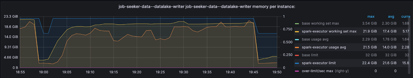
As a first attempt at recognizing an OOM error, set up your executor monitoring graphs to depict the assigned executor limit, usage average, working set max, and over limit per second. 

The below example shows a successful job where actual usage (orange / yellow) doesn’t exceed the limit we assigned to the executor (blue). Thus, the ‘over limit’ graph is zero. 

To get more detail, however, you’ll need to read your Spark job task logs. 

Of course, there may be different types of errors. In this context, we’ll focus on Excessive Memory Consumption (OOM) errors, which require us to optimize our job or adjust the config/manifest, and Lost Executor errors which are usually cascading errors when previous outputs calculated on an executor are no longer available to other executors.

While driver memory issues are typically easy to identify (by inspecting the driver pod) and solve, executor OOM errors need a bit more digging into the driver’s logs.

The errors we initially receive don’t provide much in terms of the root cause:

StreamingQueryException (Query [id = 8e57eaaf-9e92-4708-ad2e-d589cc986d23, runId = 10862bf8-7633-40c9-bf1a-4a05151dbac2] terminated with exception: Job aborted.) : SparkException (Job aborted.) : SparkException (Job aborted due to stage failure: ResultStage 310 (start at JSRTrusted.scala:48) has failed the maximum allowable number of times: 4. Most recent failure reason:
org.apache.spark.shuffle.MetadataFetchFailedException: Missing an output location for shuffle 86 partition 1527

But, by looking deeper we can find the ID of the executor, the exit code, and that indeed it was an OOM issue (137 means K8s killed the job).

Lost task 1403.0 in stage 298.0 (TID 133180) (10.68.145.23 executor 5)

…

Lost executor 92 on 10.68.148.67: 

The executor with id 92 exited with exit code 137(SIGKILL, possible container OOM).

The API gave the following container statuses:

container name: spark-executor
container image: 0123456789.dkr.ecr.us-east-1.amazonaws.com/job_seeker_data/datalake_writer:treesha-d812c2c3402228c26ad06f2760e885a448f58229-default
container state: terminated
container started at: 2023-04-24T04:39:56Z
container finished at: 2023-04-24T04:57:46Z
exit code: 137
termination reason: OOMKilled

Not sure how to find these logs? Read on. 

Finding your Spark executor logs when running on Kubernetes

Finding executor logs may seem difficult since we rarely know the name of the pod. Here are are a few ways to find your executor logs: 

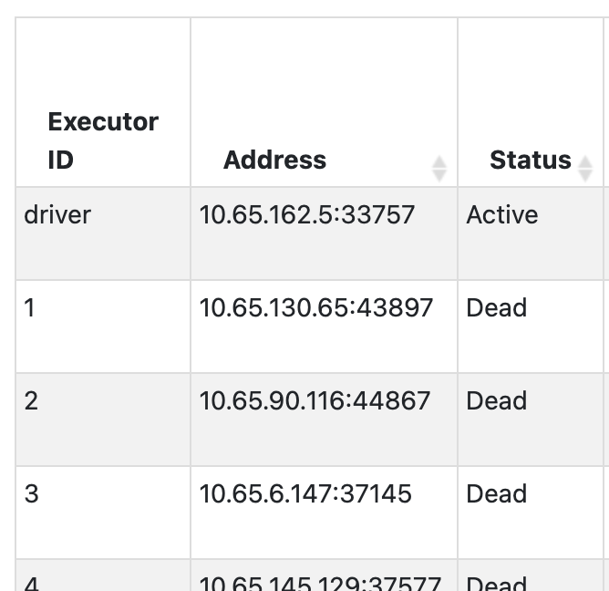
1. Open Spark UI / Spark History Server and find the IP address of the executor ID you want to check in the Executors tab:
   
   
2. Find that IP address in the logs of your Kuberbetes or equivalent cluster management solutions around the time the Spark job ran. At Ziprecruiter, we collect information on pod IPs and names from our Kubernetes clusters onto our unified logging solution.
   
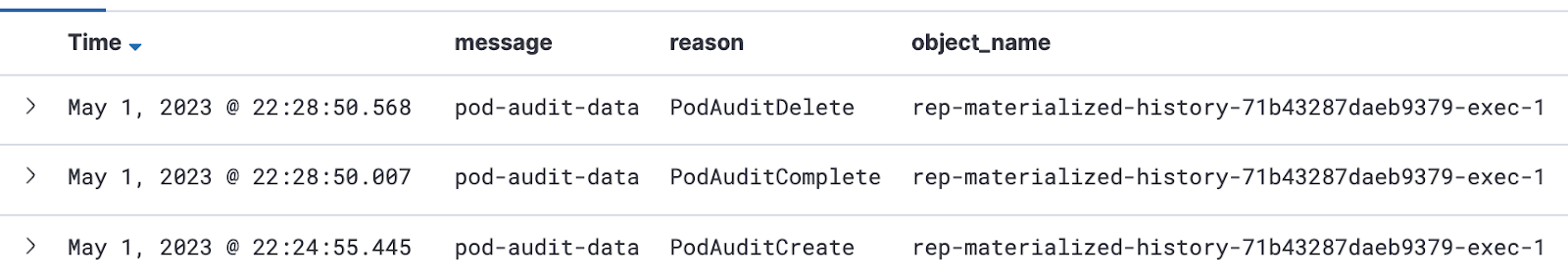
3. Take the object_name and use it as a source_host in your query to investigate. 

Improving speed and resource use of a simple Spark job

To demonstrate the systematic methodology of improving speed and resource use of a Spark job, let’s use an example. Say we want to combine multiple datasets with data about job post listings and employer campaigns (each with multiple listings) into a table of all the listings, each with their campaign data, separated to active and non-active listings. 

For the task we initially assign 10 Executors, 4 cores, and 8 GB of memory.

Here is the first shot of our code. 

val dfJoin = spark.sql(....) // run the join into a dataset
if (dfJoin.count() > 0)   // If there is data
(
dfJoin
.repartition(col("listing_status")) //group the active listings together
.write
.partitionBy("listing_status").mode("overwrite")
// write to an s3 layer partitioned by status
.parquet("...")
)
else
(  println("there is no data to write"))

It took 6 minutes to run, so let’s improve. 

Finding repartitioning bottlenecks 

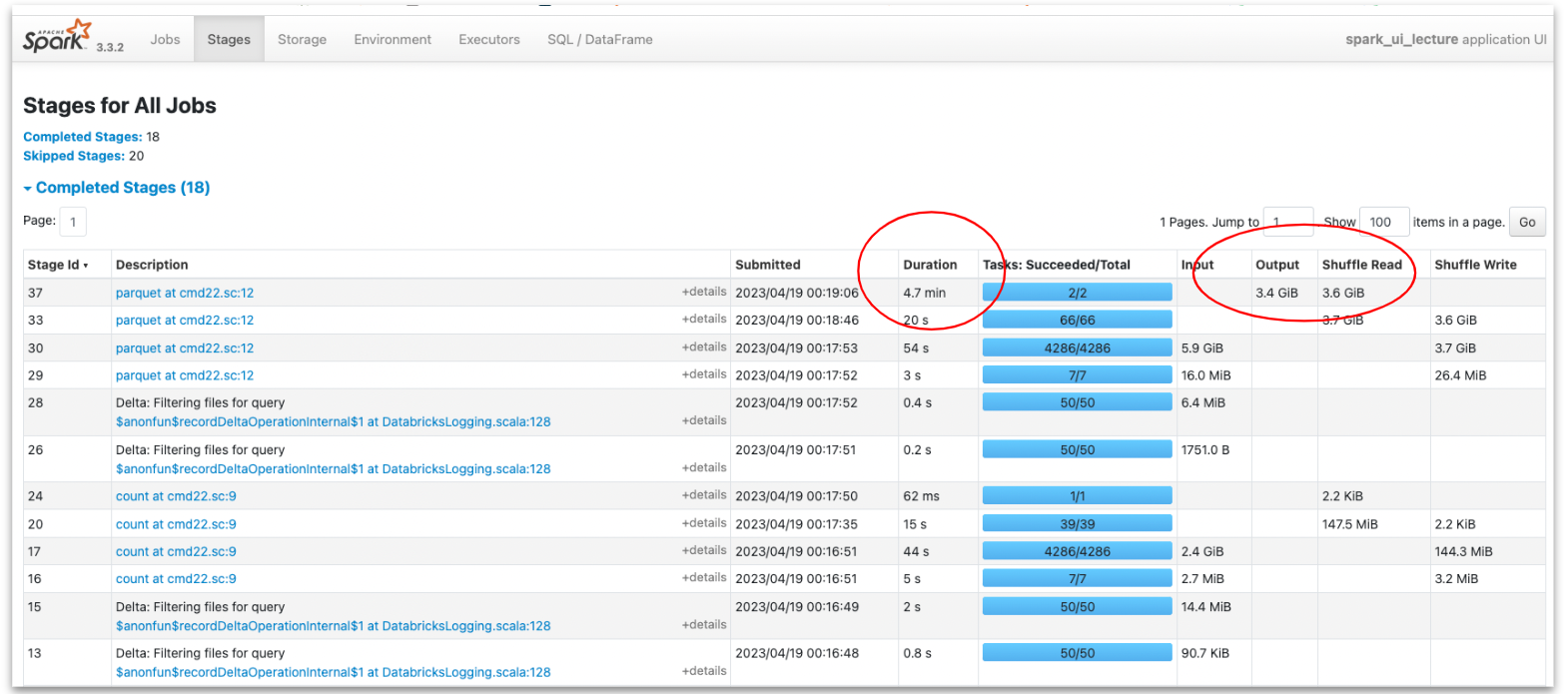
To investigate and find bottlenecks we look at the second Stages tabl in the Spark UI. This is the part in our app that either reads, shuffles, or writes data. Sorting by duration reveals the most lengthy stage. 

To understand what this stage does we look at the right hand columns. In this case, the lengthy stage of 4.7 minutes is one that spends the most time writing the data to S3. 

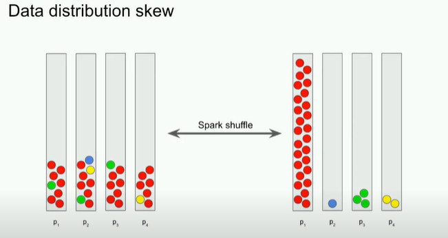
Drilling down into this stage we learn more insightful information: we only have 2 tasks instead of an expected 40 (10 executors X 4 cores) and there is a significant difference in their duration. In addition, we see we have only two files with entirely different partition sizes. This indicates data skewness – there are many more inactive listings than active ones in our data. In the future, as datasets grow, this skewness can cause our app to fail on executor memory. Lucky we caught it now in exploration! 

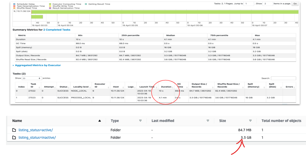
The decision to repartition the data based on the active/inactive status resulted in a serial application and under-utilization of the computation power. 

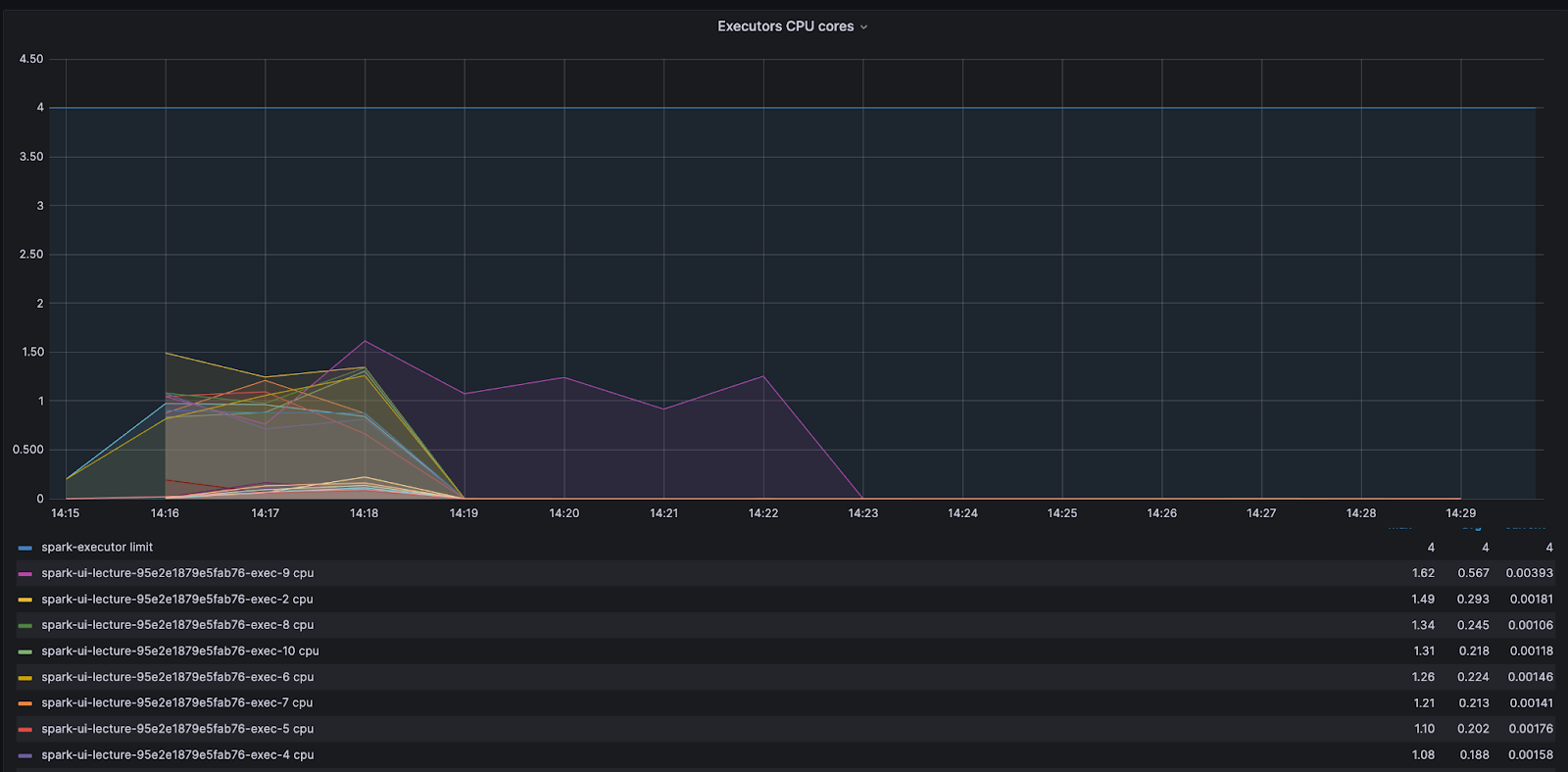
By looking at the core activity graph we can see that most cores finished early and waited in an idle state for one core. This is a clear signal of CPU waste and that adding more resources will not improve the process – the problem is with the code. 

Understanding data skew

Despite the best efforts of the Adaptive Query Enabler (AQE), which in Spark 3.2.0 or newer is active by default, data may still be skewed. And a skewed dataset means tasks working on the larger partition will take a larger amount of time to run. 

It is prudent to remember that besides inherent data shape, there are a few ways we ourselves can skew our data. There are ample resources out there on detecting and dealing with skew datasets, so let’s just state the two key types: input skew and processing skew. 

Input skew is when the data starts out or is ‘made skew’ from the beginning. For example, partitioning based on input timespan during a period of high job seeker influx. In this case one would need to repartition before the data is written. 

Processing skew. This typically happens when we need to group by or join using a skewed property in the data records, as we saw with our code above. One tip is to avoid shuffling data based on size or a very common and no-value-add attribute, like creating a partition with all job seekers who have ‘English’ as a skill. 

To fix our code let’s skip the repetition and split the data when we write it. 

if (dfJoin.count() > 0) 
(
dfJoin.repartition(col("listing_status"))
.write
.partitionBy("listing_status").mode("overwrite")
.parquet("...")
    )
else
( println("there is no data to write"))

This change cut our run time down to 38 seconds! We saved time and I/O, but there are still other problems and ways to improve. 

A small files problem – smart repartitioning

Clicking on the stage in the SparkUI reveals that now we have 200 files for just 85 MB of total data. This happens because the default amount of shuffle partitions is 200, which in our skewed data case, has created a small files problem. In S3 we usually want to create files with a minimum size of 128 MB, and in some cases even more than that. 

To avoid this problem we usually want to repartition but in a smarter way. Spark enables repartition by range, where you can determine the max amount of partitions and how you want to divide or split the data. In our case, however, where we initially had only two distinct identifiers (active/inactive) Spark would ignore a higher partition request. To overcome this we need to add a higher cardinality column such as the primary key of the data. 

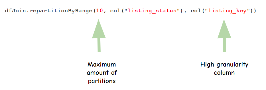
The way Spark works is that it samples a small portion of the data (default = 100 records), tries to understand how it’s distributed and only then starts the partitioning. If you have very skewed data that may not be revealed in a small sample, you will want to increase the amount of data Spark samples so it gets a better idea of your data.  

This is done by adjusting this variable:

spark.sql.execution.rangeExchange.sampleSizePerPartition

The result is an even faster run, where executors are all working to a similar extent and the output is 10 files for inactive records with much more reasonable file sizes. 

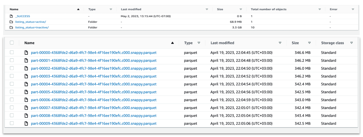
The active listings will still have smaller files as the data is skewed. But this can be fixed later using Delta Optimizer (for Deltalake tables), or we could decide to split the write and use a different repartitioning method for the active vs not active. Conversely, we may also decide not to partition to two different locations at all.

Tuning Read with maxPartitionBytes

There is also an opportunity to make the read run faster. The following config variable

spark.sql.files.maxPartitionBytes 

determines the maximum size of each partition when initially reading from files. The default value is 128MB, but for tables with files larger than 128MB it is worth increasing to larger values. In our case, the listings table holds 1GB size files and increasing this config variable to 1GB can cut over 20 seconds from our read time.

Tuning Join with broadcast

When joining between two disproportionate datasets, like campaigns (small) and job listings (large) in our case, Spark will first try to sort-merge. Namely, Spark will first sort each of the tables, then shuffle the data so the join column is in the same partition, and then try to join. 

When there is a significantly smaller table, we may save time by copying it individually into each executor and performing the join locally with each partition of a large table. The problem with this is the memory required to hold the small table. The trick here is to adjust your broadcast chunk size to take advantage of the ‘smallness’ of the small table. 

spark.sql.autoBroadcastJoinThreshold holds the default table size for broadcasting to multiple executors, and is set at 10MB. Carefully increase this to achieve improved performance. 

💡 NOTE: broadcast join is not supported in full outer joins, so if you’re using Delta merge commands with match/not-match commands then broadcast will not work. Nor does it work in anti-equal joins. 

Avoiding caching and counts to reduce memory use

In general, try to avoid actions which cause datasets to be recomputed, such as counts, collects, show, and foreach, as these drain memory severely. Instead, try to find other ways to collect metrics on your Spark apps. 

Use accumulators or just query the end result of your writing. For Deltalake tables you can also read statistics that are stored in the Delta log files, such as the amount of records and files that were written.

Finally, remember that data is not cached when the executor arrives at that line in our code. Data is only cached when an action needs to be performed that requires this dataset. This can create some unexpected behavior; for example, running a count and then later running a cache might not produce the same results because count doesn’t require all the data, it just decaches the minimum amount required to perform the count. 

By removing the count from our code we saved some more run time. 

Multiple small memory improvements have a compounding effect

The example above shows how Spark UI can help us identify issues with our code. It is, however, our responsibility as engineers to understand the nature of our data properly during exploration phases and plan ahead, so we can have context as to why Spark acts the way it does with our data. 

We must learn to identify bottlenecks and problems with our code before rushing to add CPU and memory so we can build systems that scale more efficiently, waste less memory, and ultimately cost less to our business. 

To do that, we need to understand how Spark works and not treat it as a black box.

If you’re interested in working on solutions like these, visit our Careers page to see open roles.

* * *

About the Authors: 

Naama Gal-Or is a Staff Software Engineer at ZipRecruiter. She has built a successful career centered around large-scale data applications. For over 6 years, every day at ZipRecruiter continues to provide the scale and complexity she loves while posing new and exciting challenges.

Vitaly Polonetsky is a Senior Staff Software Engineer at ZipRecruiter where he is in charge of building the systems that keep ZipRecruiter’s services running and scaling fast. He has 20 years of software developer experience, of which he has spent 7 years engulfed in big data. Vitaly loves being able to build tools for the enthusiastic engineers at ZipRecruiter, working with them one-on-one as a mentor and tech leader.